Introduction

The repositories of distributions such as Debian and Nixpkgs are among the largest collections of open source (and some unfree) software. They are complex systems that connect and organize many interdependent packages. Interestingly, these systems grow out of the individual design choices of thousands of contributors but few of them have larger design goals in mind.

Is it possible to capture the large scale features of such a repository in an image? Are there common design choices of the contributors? Did they lead to any emergent structure?

Plenty of studies (e.g. here, here, or here) have examined these questions from different viewpoints and for various software ecosystems. In this blog post I’ll try to shed some light on them from the perspective of Nixpkgs, mostly with visualizations of its complete dependency graph but also with a very short examination of its statistical properties (its degree distribution). But wait, you might think: “visualizing a graph with 50000 nodes and 300000 edges? - All you are going to see is black!“. Well, it turns out that this is not the case because large scale structures appear when we look at the graph in the right way.

An overview of the Nixpkgs dependency graph

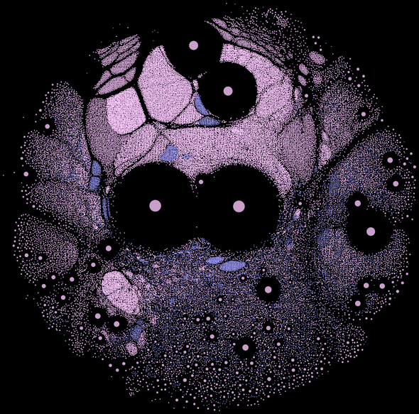
Before explaining in detail what I did, let’s start with a teaser. Check out the structure in this fascinating image where each little dot represents a single software package in the Nixpkgs repository:

What looks remotely like the section of a mouse brain actually represents around 46000 software packages. Each dot in this image corresponds to a different one, more precisely to a Nix derivation in the Nixpkgs repository. Each package is invisibly linked to those that it depends on (ingoing dependencies) or those that depend on it (outgoing dependencies). These packages are the nodes, and their invisible links the incoming and outgoing edges of the directed dependency graph of Nixpkgs.

The total number of dependencies that a node has is called the node’s degree. It is subdivided in the in degree which counts the number of ingoing dependencies and the out degree which counts the number of outgoing dependencies. I have colored and sized the nodes in the above image by their in degree: a brighter larger node means that more derivations depend on it (high in degree) than on a darker smaller node (low in degree). Size and color are scaled non-linearly and should only be interpreted qualitatively. We will see later from the distribution of these degrees why this makes sense.

The graph was laid out and visualized with the program gephi using a force simulation algorithm to project each node to a display positions in the image. This force model consists of attractive and repulsive forces that drag the nodes into their final positions that you can see in the image.

The attractive force pulls nodes towards their dependencies. Therefore nodes with similar dependencies end up close to each other. Looking back at the image, we see the effect of this force in the form of node clusters with visible gaps between them. The repulsive force pushes nodes away from dependencies that have high degree. High degree nodes therefore appear with a lot of space around them. Low degree nodes, on the other hand, are tightly packed.

As a final addition, a gravitational force keeps the whole graph together and squeezes it into roughly circular form. Check out the appendix at the end of this post for a detailed explanation, including the code and the data that are required to reproduce this image yourself.

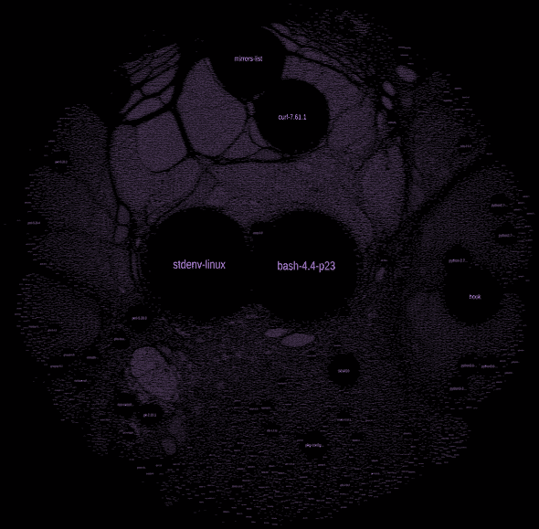
The following image of the dependency graph was laid out in the same way, but shows the package name of each node explicitly. As before, the package names are scaled non-linearly with the in degree of the node. The names of the largest nodes - we’ll call them hub nodes - are well readable but to read the labels of the smaller nodes you should click on the image and use your browsers zoom functionality.

Most central to the Nixpkgs repository are the primary hub nodes bash and the Nix stdenv derivation. Unsurprisingly, most derivations depend on them - at least at build time - because bash is one of the most commonly used Unix shells and stdenv is a nix package that groups very fundamental build dependencies such as GNU make. Both are used as default environments in Nix.

Slightly smaller secondary hub nodes can also be identified: curl and mirrors-list seem to be central to the upper part of the graph and indicate that it has something to do with the internet. On the right side, Python2.7 and Python3.6 are visible as distinct clusters and grouped around a central hook derivation that is used by Nix to setup a Python environment. On the left side, different versions of Perl can be seen. In the bottom, the Linux library manager tool pkg-config forms a little aura that matches its importance for the open source ecosystem.

The hub nodes indicate that some clusters in this graph correspond to the environments of different programming languages. Naturally packages in these environments will have a common set of dependencies and therefore appear close to each other in the graph.

Ego networks: exploring hub node environments

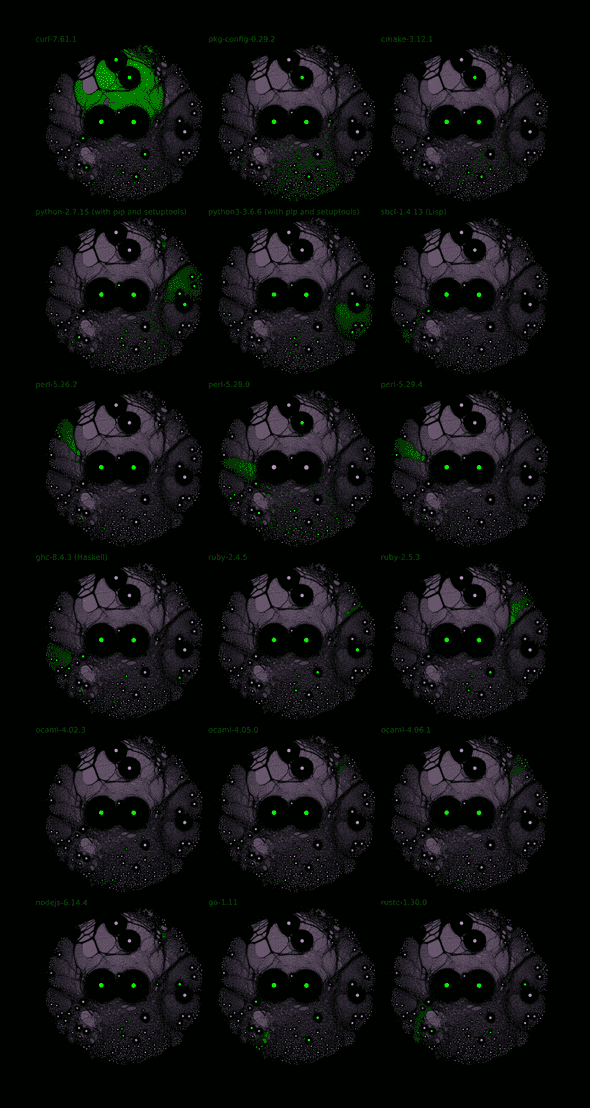
Let’s dive further into this. A hub node forms a little subgraph together with its ingoing and outgoing dependencies that is sometimes called its ego network (this term seems to originate in studies of social networks). In the following plot, the ego networks of a few selected hub nodes are colored in green. The corresponding hub node’s name is indicated above each subplot. It illustrates nicely how clusters form around a compiler, an interpreter or just an important tool:

The ego networks confirm our previous intuition that some clusters correspond to different programming languages. They also provide basic orientation on this graph. Here is a short description of the different ego networks:

Most of the upper part of the graph is dominated by curl. Closer inspection shows that most of these derivations are archives such as .tar.gz files or language specific archives such as .gem files. These archives are downloaded from the internet before other packages are derived from them. Another large, but less tightly packed region is the pkg-config zone. It dominates the bottom of the graph and it is characterized by lots of smaller hub nodes indicating that pkg-config organizes many packages that are important for other packages. The ego network of cmake is mixed into a similar region of the graph.

Python2.7 and Python3.6 form neat clusters with three central hub nodes that correpond to the python interpreter, the package management tool pip, and the build and installation tool setuptools. Python2.7 is used more often by packages outside of its cluster than Python3.6. In contrast to Python, Perl has only a single hub node for each specific version but it forms similarly dense clusters. From the different Perl versions, Perl-5.28.0 is reused most outside of its own cluster by a lot of other packages in the pkg-config zone. This indicates that the specific version of the Nixpkgs repository that I have evaluated uses this particular Perl version as the default for other packages.

Lisp (sbcl), Haskell (ghc), Ruby, OCaml, Go, and Rust derivations also accumulate in tight clusters around their respective compiler.

Ego networks can only give a glimpse into the structure of the graph of Nixpkgs. Not all environments are organized around a central hub. Some packages are self-contained and independent. For example, the Go packages form a tight independent group because they often include copies of third party packages that they depend on. There are also many smaller clusters that correspond to particular tools such as terraform, maven or even the vim plugins. If you have time and patience, you can try to find them in the labelled graph image above.

The degree distribution of the Nixpkgs dependency graph

Another perspective on the global properties of the Nixpkgs repository is the degree distribution of its nodes. It shows how many nodes exist with a certain in or out degree (as a reminder: the in degree is the number of packages that depend on the node; the out degree is the number of packages that the node depends on). Certainly there are a lot more nodes with low in degree than with high in degree. More interesting is how the number of nodes with a certain degree changes between the extremes.

A whole bunch of studies (for example here, here) have found that the in degree distribution of software repository dependencies follows a power-law distribution, similar to the degree distributions of networks in Geology, Biology, Economics, or the Internet (here is a short introduction on power-laws). Such a power-law distribution can be generated by several mechanisms. The hottest candidate mechanism in the case of software repositories seems to be preferential attachment, a.k.a. “the rich get richer”. In other words, a new package is more likely to depend on existing packages with a lot than on packages with few dependencies. Other mechanisms such as self-organized criticality might also play a role.

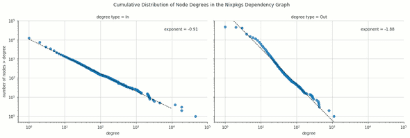
The (complementary) cumulative in and out degree distributions show how many packages exist above a certain degree. Looking at the cumulative distribution is typically better than looking at its derivative, the degree distribution. As an integral, the cumulative distribution has a better behavior when the density of packages gets low at high degrees. We plot it here for the in and out degrees in log-log scale such that a power-law is just a straight line:

The cumulative in degree distribution is a very clean power-law decay with an exponent of -0.9. The in degree distribution itself has an exponent of -1.9, because it is the derivative of the cumulative distribution. The value that we observe falls in the range of values that have been observed for the debian repository (around -2.0). Interestingly, a power-law distribution is also a scale-free distribution: For example, at the largest scale of Nixpkgs, a node with an approximate (order of magnitude) in degree of 2000 such as a python2.7 (3033), perl-5.28 (2406), or git (2394), is about 80 times (=10^1.9) less common than a node with in degree 200, which could be an important library such as python2.7-mock (212), python3.6-six (321), or freetype (303). On the other hand, such a node with degree 200 is also about 80 times less common than a node with approximate in degree 20, such as python3.6-flake8 (23), ruby2.5.3-nokogiri (20), or erlang (19). In some sense, the large scale ecosystems around python, perl, or git are therefore scaled up versions of the small scale ecosystems around a minor programming language or library. This shows that there is more to a software repository such as Nixpkgs than just a few primary and secondary hub nodes. It is a complex growing ecosystem.

The out degree of a package counts how many other packages the node depends on. Its cumulative distribution looks a bit different than the one for the in degrees. It has a cutoff at around degree 3, which means that only few nodes depend on three or less packages. At degree 4, the distribution drops markedly, which means that there are lots of packages that depend on 4 other packages. The decay afterwards is also not quite as regular as for the in degrees. If we interpret this decay as a power-law, the decay rate corresponds to an exponent of around -2.9. This means that a node that depends on 200 packages is about 800 times (=10^2.9) less common than a node that depends on 20 packages. Although this gives some intuition about the out degree distribution, it is unclear if a power-law is really a good model for it. Preferential attachment is less plausible as generating mechanism behind the out degree distribution because the number of dependencies that a package depends on is often directly chosen by the developers. Other distributions, such as multiple overlapping log-normals, could potentially fit the distribution equally well and also account for different mechanisms.

Conclusions

The graph visualizations give an overview of the structure of the enormous Nixpkgs repository that can be difficult to grasp in its entirety otherwise. The degree distribution of the nodes is another macro perspective of the repository that is difficult to obtain with other means. It would also be interesting to examine whether the degree distributions of different language environments differ. Taking a step back, I hope that this blog post can raise some awareness for the complexity and beauty of a system that was generated by thousands of individual contributions but that ultimately becomes more than the sum of its parts.

Appendix: do it yourself

If you want to explore the Nixpkgs dependency graph yourself, you can download the gephi project file that will allow you to start immediately. The Nixpkgs graph in dot format can be used with graphviz and many other libraries. Finally, I have also uploaded the Nixpkgs graph as a sparse adjacency matrix.

You can also regenerate the graph from the beginning:

A Nix derivation is a recipe with all meta information that is required to build a package. This includes links to other required derivations, hashed source code, shell commands, compiler flags, environment variables, and so on. Derivations are not written by hand but generated automatically by evaluating code that is written in the Nix language. The Nixpkgs repository is a collection of such Nix code and generates by default around 46000 derivation files with build recipes. These derivation files are stored as human readable text files with the extension .drv in the Nix store folder (usually under /nix/store).

To build the dependency graph, I traversed and evaluated the whole Nixpkgs repository with a few lines of Nix code. This process is quite fast (<5min) because no package has to be actually built. The derivation files only gather the meta information that is needed to build them. I then extracted the package dependencies from each derivation file in the store with a small Haskell code and saved them as a graph .dot file (here is the Nix and Haskell code). Due to the graph’s size, I merged derivations with the same package and version name, ignoring other build characeristics that are typically identified with a unique hash by Nix.

The graph was laid out and visualized with the program gephi using a force simulation algorithm to project the graph nodes to display positions in the image. The simulation starts by putting the nodes at random initial positions. Afterwards it updates the node positions stepwise according to a force model until they find a steady place. The force model, called Force Atlas 2, consists of an attractive and of a repulsive force between connected nodes. The attractive force is proportional to the distance and the repulsive force inversely proportional to the distance of the connected nodes. In addition, the repulsive force is proportional to the product of the degrees of the connected nodes, that is to the number of edges that are incident on them. The nodes are therefore pushed to an equilibrium distance where the forces are balanced. The equilibrium distance is smaller for nodes with low degree and larger for nodes with high degrees.

Getting a nice visualization is then a matter of fine-tuning the corresponding parameters of the force simulation in gephi, together with the color scheme and the node sizes, until the structure of the graph becomes most evident.