In a recent blog post, we analyzed the most obvious patterns in Haskell and Python source code, namely import statements and LANGUAGE pragmas.
As promised in that blog post, let us now explore what unknown patterns are hidden in our data sets.
To this end, we will create two-dimensional “maps” of code, which allow for a nice visualization of code patterns and may make you appreciate the beauty and complex structure of the code you and your friends and colleagues write.
Such code patterns also provide insight into the coding habits of a community in a programming language ecosystem.
We will conclude this blog post with an outlook on how these and similar patterns can be exploited.
Quantitative representation of source code
The sort of patterns that we are looking for is some kind of similarity between lines of codes. While the concept of similarity between two lines of code might be intuitively clear for us humans, we don’t have time to print out a large number of lines of code on little snips of paper and sort them in piles according to their similarity. So obviously, we want to use a computer for that. Unfortunately, computers a priori don’t know what similarity between two lines of code means.
To enable computers to measure similarity, a first step is to represent each line of code as a vector, which is a quantitative representation of what we think are the most important characteristics (“features”) of a line of code. This is a common task in Natural Language Processing (NLP), which is concerned with automatic analysis of large amounts of natural language data. While the languages we are considering are not natural, but constructed, we expect key concepts to be transferable. We thus borrow the idea of a bag-of-words from NLP: for a given line of code, we neglect grammar and word order, but keep a measure of presence of each word. In our case, we only take into account the 500 most frequent words in our data set and simply check which of these words is present in a line of code and which are not. That way, we end up with a 500-dimensional feature vector, in which each dimension encodes the occurrence of a word: it’s either one (if the word is present in that line of code) or zero (if it is not).
Visualizing source code
We could now race off and compare all these representations of lines of code in the 500-dimensional feature space. But do all of these dimensions really contain valuable information which sets apart one pattern from another? And, how would we visualize such a high-dimensional space?
A popular way to address these questions is to reduce the number of dimensions significantly while keeping as much information about the structure of the data as possible. For the purpose of visualization, we would love to have a two-dimensional representation so that we can draw a map of points in which points with similar features are placed close to each other and form groups (“clusters”). To achieve that, we need a measure of similarity (or, equivalently, distance) in feature space. Here, we define similarity between two lines of code by the number of words they have in common: we count the number of unequal entries of two feature vectors and the lower that number is, the lower is the so-called Hamming distance between the two feature vectors and the more similar they are.
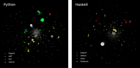
A popular technique to reduce the number of dimensions while trying to maintain the structure of the data or, equivalently, the distances between similar data points, is UMAP. We first use UMAP to calculate a two-dimensional map of both the Python and the Haskell data set and color points depending on whether the line of code they represent contain certain keywords:
We immediately notice the complex structure of the data set, which seems to consist of a large number of clusters comprising very similar lines of code. We expect many lines of code containing the keywords we chose to be close together on the UMAP which is indeed what we observe, although they do not necessarily form connected clusters. Furthermore, one line of code could contain several of the keywords, which would not be visible in our representation.
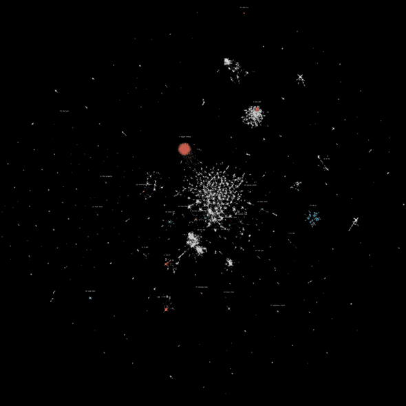
To find out what kind of code other clusters represent, we perform clustering on the UMAP embedding, meaning that we run an algorithm on the map which automatically determines which points belong to which cluster. Starting with the Python data set, we annotate the twenty most dense and reasonably large clusters with the two words which co-occur most frequently in a cluster:
We are not surprised to find clusters with the most frequent words being for and in, which corresponds to Python for-loops, or assertEqual and self, which stems from the unittest framework. Some other clusters, though, do not remind us of common Python idioms. The most common words in cluster 17 are xd and xc. Looking up what kinds of lines of code contain both of these words, we find that these occur very often in byte strings. In our earlier blog post we already learned that in Haskell, byte strings feature prominently in a few select packages.
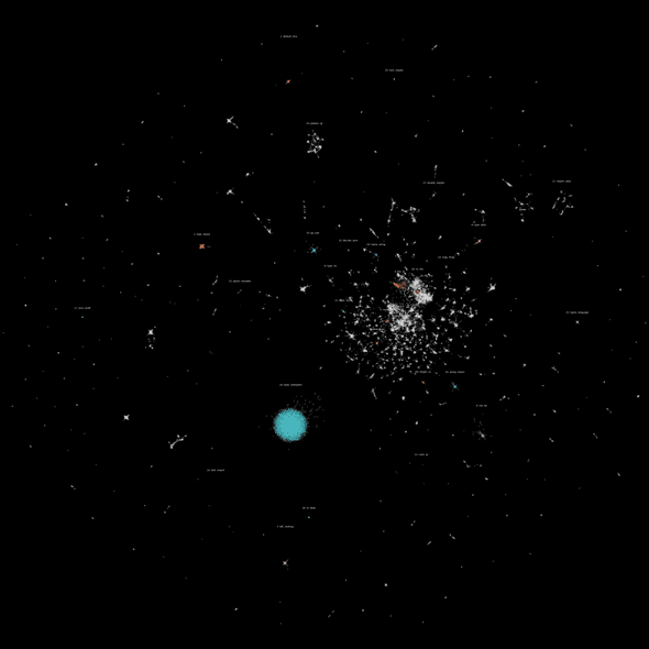
Performing the same analysis for the Haskell data set, we find clusters such as a very well-defined one containing often both text and maybe and clusters corresponding to popular imports:
Furthermore, the big blue cluster (#16) seems to contain mostly auto-generated code from the amazonka package, which implements communication with Amazon Web Service-compatible APIs.
Conclusion
We found several interesting patterns in both Haskell and Python code—clusters of common language idioms, but also unexpected clusters stemming from byte strings. With these results, we could now build a very basic code completion tool: while you type, that tool would continuously check to which cluster the line you’re typing most likely belongs to and suggest you words from that cluster. An obvious limitation, though, is the complete absence of context-sensitivity, meaning that proposed words neither depend on the order of previous words in the same line nor on adjacent lines of code.
Other projects have taken the application of machine learning techniques much further, resulting in tools which can significantly facilitate programmers’ lives. Kite performs context-sensitive code completion for Python and is available as a plug-in for several popular IDEs. The Learning from Big Code website lists several other interesting projects. For example, the Software Reliability Lab at ETH Zurich developed JSNice, a tool to automatically rename and deobfuscate JavaScript code and to infer types. Finally, Naturalize learns coding conventions from an existing codebase to improve consistency.
Appendix: data preprocessing and technical details
We limited our analysis on 100,000 randomly chosen lines of code, which we tokenized, meaning we replace all types of whitespace by a single space, retained only letters and converted upper case letters to lower case ones.
To perform a dimensionality reduction of our data sets, it is necessary to create informative feature vectors from each line of code.
We used count vectorization as implemented in scikit-learn to turn each line of code in a binary vector, whose dimensions correspond to the 500 most frequent words in our Python / Haskell code corpus.
We don’t care how often a word occurs in a line of code, only whether it’s there (1) or not (0).
Furthermore, single-letter words are neglected.
Having built these feature vectors, we applied a popular dimensionality reduction technique, UMAP. UMAP is a manifold embedding technique, meaning that it tries to represent each data point in the high-dimensional feature space by a point on a lower-dimensional manifold in a way that similar points in the feature space lie close together on the lower-dimensional manifold. It is a non-linear mapping, which means it’s well suited for data sets which can not easily be projected on flat manifolds. UMAP requires a measure of similarity in feature space, which we chose as the Hamming distance between two binary feature vectors.
To assign points in the two-dimensional representations of our data sets to clusters, we used the Python implementation of the recent clustering algorithm HDBSCAN (paywalled). A big advantage of HDBSCAN over many other clustering algorithms is that it automatically determines the number of clusters and allows to classify data points as noise.


