This is part 4 of a series of blog posts about MCMC techniques:

• Part I: The basics
• Part II: Gibbs sampling
• Part III: Hamiltonian Monte Carlo

In the previous three posts, we covered both basic and more powerful Markov chain Monte Carlo (MCMC) techniques. In case you are unfamiliar with MCMC: it is a class of methods for sampling from probability distributions with unknown normalization constant and to make the most of this post, I would recommend to get acquainted with MCMC basics by, for example, reading the first post of this series.
The algorithms we discussed previously already get you quite far in everyday problems and are implemented in probabilistic programming packages such as PyMC3 or Stan. In the (for now) final post of this series, we will leave behind the MCMC mainstream and discuss a technique to tackle highly multimodal sampling problems.

As we saw in the Gaussian mixture example in the Gibbs sampling blog post, a Markov chain can have a hard time overcoming low-probability barriers in the limited time we are simulating it. Such a stuck Markov chain thus samples a distribution incorrectly, because it oversamples some modes and undersamples others.
A cool way to overcome this problem is to not simulate only from the distribution of interest, but also flatter versions (“replicas”) of it, in which low-probability regions can be crossed more easily. If we then occasionally exchange states between these flatter Markov chains and the Markov chain sampling the distribution of interest, the latter chain will eventually get unstuck, as incoming states from flatter distributions are more likely to be located in a different mode. This is the principal idea of Replica Exchange (RE), also known as “Parallel Tempering” (PT) or “Metropolis Coupled Markov Chain Monte Carlo”.

Replica…

Just as several other MCMC algorithms, RE has its origins in computational physics and just as before, we will help ourselves to some physics terminology.
As discussed in the previous blog post about Hamiltonian Monte Carlo, under certain conditions, the probability for a physical system to be in a certain state $x$ is characterized by a potential energy $E(x)$ and given by $p(x)\propto\exp[-E(x)]$. In fact, for simplicity, we omitted a little detail: the system has a temperature $T$, which influences the probability of the state $x$ via a constant $\beta \propto \frac{1}{T}$. The complete formula for the probability is then

The temperature is important, as it essentially determines the “flatness” of the distribution $p_\beta(x)$. In a high-temperature system (meaning $\beta \approx 0$), energy barriers can be easily crossed because $p_\beta(x)$ is almost uniform. Physically speaking, because particles move very fast at high temperatures, they can overcome forces acting on them more easily.
Therefore, parameterizing the distribution $p(x)$ by $\beta$ in the above way gives us exactly what we need for RE: a family of distributions (replicas), which are increasingly flatter and thus easier to sample. This family of distributions is given by $p_\beta(x)=p(x)^\beta$ with $1 \geq \beta \geq 0$ and $p_1(x)=p(x)$ being the distribution we’re actually interested in. We call the distributions with $\beta < 1$ “tempered”. Let’s take up again the example of a Gaussian mixture and make some choice of inverse temperatures:

mix_params = dict(mu1=-1.5, mu2=2.0, sigma1=0.5, sigma2=0.2, w1=0.3, w2=0.7)
mixture = GaussianMixture(**mix_params)
temperatures = [0.1, 0.4, 0.6, 0.8, 1.0]

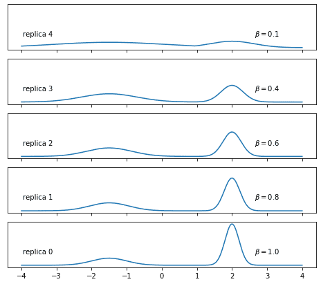
What do the tempered mixtures looks like? Let’s plot them:

I believe that you’ll agree that the upper distributions look somewhat easier to sample. Note, though, that this is not the only way to obtain a family of tempered distributions.

… Exchange

Now that we know how to obtain flatter replicas of our target density, let’s work out the other key component of Replica Exchange — the exchanges between them. Naively, you would probably do the following: if, after $k$ steps of sampling, the Markov chain $i$ is in state state $x^i_k$ and the Markov chain $j$ is in state $x^j_k$, then an exchange of states between the two chains leads to the next state of chain $i$ being in state $x^i_{k+1}=x^j_k$, while chain $j$ will assume $x^j_{k+1}=x^i_k$ as its next state.¹
Of course you can’t just swap states like that, because the exchanged states will not be drawn from the right distribution. So what do we do if we have a proposal state which is not from the correct distribution? The same thing we always do: we use a Metropolis criterion to conditionally accept / reject it, thus making sure that the Markov chain’s equilibrium distribution is maintained. So the probability to accept the exchange is the probability to accept the new proposal state in chain $i$ ($p_{j\rightarrow i}$) times the probability to accept the new proposal state in chain $j$ ($p_{i\rightarrow j}$). Here’s the full expression for the exchange acceptance probability:

Some thought has to be put into how to choose the replica pairs for which exchanges are attempted. Imagine having three replicas. In a single exchange attempt, only two replicas, say, $2$ and $3$, are involved, while the target distribution, sampled by replica $1$, performs a regular, local MCMC move instead. After attempting an exchange between replicas $2$ and $3$, all replicas would continue to sample locally for a while until it’s time for the next exchange attempt. If we chose again replicas $2$ and $3$ and kept on doing so, replica $1$ would not be “connected” to the other two replicas. The following figure, in which each local MCMC sample is denoted by a dash and samples involved in an exchange are shown as solid dots shows how that would look like:

As the lower (target) replica doesn’t participate in any exchanges, it would likely stay stuck in its current mode. This strategy thus defeats the purpose of RE. Only if we also attempt exchanges between replica $1$ and, for example, replica $2$, replica $1$ has access to states originally stemming from the high-temperature replica $3$. That way, we make sure that all replicas are connected to each other. We best swap only replicas adjacent in the temperature ladder, because acceptance rate will decrease if the distributions are too different. That swapping strategy would look as follows:

If a replica is not participating in a swap, we just draw a normal sample. As it was the case for the tempered replicas, also the exchanges do not necessarily have to be performed in the way presented here: there is a certain freedom in choosing the acceptance criterion as well as in the scheme to select swap partners.

Implementation

Let’s implement this (for brevity, the handling of the border cases is not shown, but the full code is available in the notebook):

def build_RE_chain(init, stepsizes, n_total, temperatures, swap_interval, log_prob):

    from itertools import cycle

    n_replicas = len(temperatures)

    # a bunch of arrays in which we will store how many
    # Metropolis-Hastings / swap moves were accepted
    # and how many there were performed in total

    accepted_MH_moves = np.zeros(n_replicas)
    total_MH_moves = np.zeros(n_replicas)
    accepted_swap_moves = np.zeros(n_replicas - 1)
    total_swap_moves = np.zeros(n_replicas - 1)

    cycler = cycle((True, False))
    chain = [init]
    for k in range(n_total):
        new_multistate = []
        if k > 0 and k % swap_interval == 0:
            # perform RE swap
            # First, determine the swap partners
            if next(cycler):
                # swap (0,1), (2,3), ...
                partners = [(j-1, j) for j in range(1, n_replicas, 2)]
            else:
                # swap (1,2), (3,4), ...
                partners = [(j-1, j) for j in range(2, len(temperatures), 2)]
            # Now, for each pair of replicas, attempt an exchange
            for (i,j) in partners:
                bi, bj = temperatures[i], temperatures[j]
                lpi, lpj = log_prob(chain[-1][i]), log_prob(chain[-1][j])
                log_p_acc = min(0, bi * lpj - bi * lpi + bj * lpi - bj * lpj)
                if np.log(np.random.uniform()) < log_p_acc:
                    new_multistate += [chain[-1][j], chain[-1][i]]
                    accepted_swap_moves[i] += 1
                else:
                    new_multistate += [chain[-1][i], chain[-1][j]]
                total_swap_moves[i] += 1
            # We might have border cases: if left- / rightmost replicas don't participate
            # in swaps, have them draw a sample
            # [ full code in notebook ]
        else:
            # perform sampling in single chains
            for j, temp in enumerate(temperatures):
                accepted, state = sample_MH(chain[-1][j], lambda x: temp * log_prob(x), stepsizes[j])
                accepted_MH_moves[j] += accepted
                total_MH_moves[j] += 1
                new_multistate.append(state)
        chain.append(new_multistate)

    # calculate acceptance rates
    MH_acceptance_rates = accepted_MH_moves / total_MH_moves
    # safe division in case of zero total swap moves
    swap_acceptance_rates = np.divide(accepted_swap_moves, total_swap_moves,
                                      out=np.zeros(n_replicas - 1), where=total_swap_moves != 0)

    return MH_acceptance_rates, swap_acceptance_rates, np.array(chain)

Before we can run this beast, we have to set stepsizes for all the single Metropolis-Hastings samplers:

stepsizes = [2.75, 2.5, 2.0, 1.75, 1.6]

Note that the step size decreases: the more pronounced the modes are, the lower a step size you need to maintain a decent Metropolis-Hastings acceptance rate.
Let’s first run the three Metropolis-Hastings samplers independently by setting the swap_interval argument of the above function to something bigger than n_total, meaning that no swap will be attempted:

def print_MH_acceptance_rates(mh_acceptance_rates):
    print("MH acceptance rates: " + "".join(["{}: {:.3f} ".format(i, x)
                                             for i, x in enumerate(mh_acceptance_rates)]))


mh_acc_rates, swap_acc_rates, chains = build_RE_chain(np.random.uniform(low=-3, high=3,
                                                                        size=len(temperatures)),
                                                      stepsizes, 10000, temperatures, 500000000,
                                                      mixture.log_prob)
print_MH_acceptance_rates(mh_acc_rates)

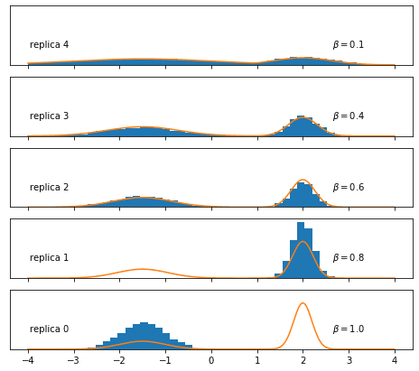
MH acceptance rates: 0: 0.794 1: 0.558 2: 0.559 3: 0.397 4: 0.704

Let’s visualize the samples:

We find, as expected, that the replicas with lower inverse temperature are sampled much more exhaustively, while the Metropolis-Hastings sampler struggles for $\beta=1$ and perhaps already $\beta = 0.8$.
Now we couple the chains by replacing every fifth Metropolis-Hastings step by an exchange step:

init = np.random.uniform(low=-4, high=4, size=len(temperatures))
mh_acc_rates, swap_acc_rates, chains = build_RE_chain(init, stepsizes,
                                                      10000, temperatures, 5,
                                                      mixture.log_prob)
print_MH_acceptance_rates(mh_acc_rates)
swap_rate_string = "".join(["{}<->{}: {:.3f}, ".format(i, i+1, x)
                            for i, x in enumerate(swap_acc_rates)])[:-2]
print("Swap acceptance rates:", swap_rate_string)

MH acceptance rates: 0: 0.798 1: 0.573 2: 0.559 3: 0.525 4: 0.501
Swap acceptance rates: 0<->1: 0.596, 1<->2: 0.827, 2<->3: 0.858, 3<->4: 0.883

It looks like the temperatures we chose are (in this case, even more than) close enough to allow for good swap acceptance rates—a necessary condition for a RE simulation to be useful.
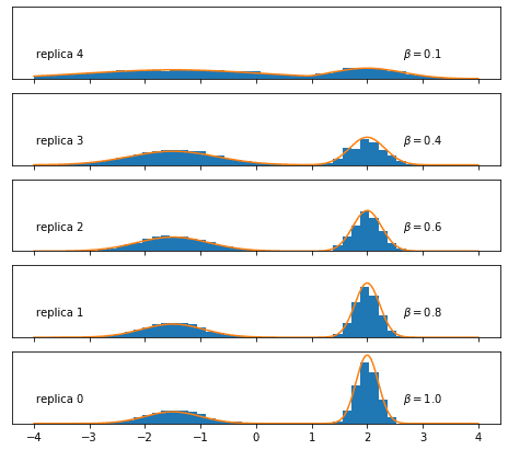
Let’s see whether the many accepted exchanges actually helped the Markov chain at $\beta=1$ to sample the target distribution exhaustively:

Et voilà! Thanks to coupling the replicas, we manage to sample correctly even at $\beta=1$!

A nice way to think about what is happening in the course of a RE simulation is to look at what happens to the initial state of a replica. The initial state will be evolved through some “local” sampling algorithms for a few steps until an exchange is attempted. If the exchange is successful, the state moves up or down a step on the “temperature ladder” and is evolved on that step until at least the next attempted exchange.
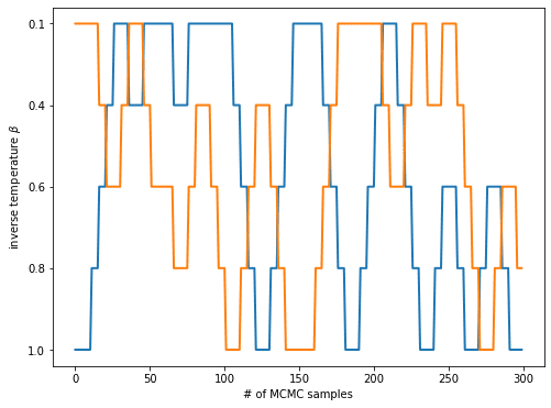
We can visualize that by first detecting, for each pair of replicas, at which simulation time points a successful swap occurred and then reconstructing the movement of a state from the list of swaps. This yields, for each initial state, a trajectory across the temperature ladder. The code for reconstructing the trajectories is skipped here, but can be found in the notebook. For clarity, we only plot the trajectories of the initial states of the target and the flattest replica:

By following the initial state of the $\beta=0.1$ chain and checking when it arrives at $\beta=1$, you can estimate how long it takes for a state to traverse the temperature ladder and potentially help the simulation at $\beta=1$ escape from its local minimum.

Drawbacks

If what you read so far leaves you amazed about the power of RE, you have all the reason to! But unfortunately, nothing is free in life…
In the above example, the price we pay for the improved sampling of the distribution at $\beta=1$ is given by the computing time expended to simulate the replicas at $\beta < 1$. The samples we drew in those replicas are not immediately useful to us.

Another issue is finding an appropriate sequence of temperatures. If your distribution has many modes and is higher-dimensional, you will need much more than one interpolating replica. Temperatures of neighboring replicas need to be similar enough as to ensure reasonable exchange rates, but not too similar in order not to have too many replicas.
Furthermore, the more replicas you have, the longer it takes for a state to diffuse from a high-temperature replica to a low-temperature one—states essentially perform a random walk in temperature space.

Finally, RE is not a mainstream technique yet—its use has mostly been limited to computational physics and biomolecular simulation, where computing clusters are readily available to power this algorithm. This means that there are, to the best of my knowledge, no RE implementations in major probabilistic programming packages. The exception is TensorFlow Probability. Seeing that PyMC4, the successor to the very popular PyMC3 probabilistic programming package, will have TensorFlow Probability as a backend, we can hope for a GPU-ready RE implementation in PyMC4.

Conclusion

I hope I was able to convince you that Replica Exchange is a powerful and relatively easy-to-implement technique to improve sampling of multimodal distributions. Now go ahead, download the notebook and play around with the code! Things you might be curious to try out are varying the number of replicas, the temperature schedule or the number of swap attempts. How are those changes reflected in the state trajectories across the temperature ladder?
If you want to take a deeper dive into RE, topics you might be interested in are histogram reweighting methods, which allow you to recycle the formerly useless samples from the $\beta<1$ replicas to calculate useful quantities such as the probability distribution’s normalization constant, or research on optimizing the temperature ladder (see this paper for a recent example).

This concludes my introductory MCMC blog post series. I hope you now have a basic understanding of both basic and advanced MCMC algorithms and specific sampling problems they address. The techniques you learned are becoming more and more popular, enabling wide-spread use of Bayesian data analysis methods by means of user-friendly probabilistic programming packages. You are now well-equipped with the necessary background knowledge to use these packages and ready to tackle your own complex data analysis problems with powerful sampling techniques!